RStudio
renv::init() # Initialize the project
renv::restore() # Download packages and their version saved in the lockfileReal-world analytical problems are often complex, making it difficult to define or derive deterministic solutions. Two common approaches to support complex analytical projects are:
While the first approach has many advantages, there are circumstances where approximating a problem with a known distribution is computationally prohibitive, overly reductive, or infeasible. In such cases, we leverage abstract probabilistic and statistical concepts to transform randomness into inferential statistics. When applied correctly, these concepts can surprisingly guarantee robust solutions to otherwise unsolvable problems.
One of these powerful techniques is Markov chain Monte Carlo (MCMC). Random samples generated with MCMC can be used for various purposes, including computing statistical estimates, numerical integrals, and estimating the marginal or joint probabilities of multivariate distributions and densities 1. Notably, MCMC provides a means to generate samples from joint distributions by utilizing conditional, factorized distributions 1,2.
Two common MCMC implementations are Metropolis-Hastings (M-H) and Gibbs sampling, with the latter being more accurately considered a special case of the former. Students are encouraged to explore M-H further on their own by reading the relevant sections of the supporting textbooks listed below. Today, we will focus on Gibbs sampling and only discuss M-H where it supports this learning, as Gibbs sampling is particularly well-suited for reducing high-dimensional problems into several one-dimensional ones 1,3.
The concepts discussed here have been compiled and summarized from various resources listed in the bibliography at the end of this page. We would like to specifically highlight the following textbooks, with suggested readings, or online course materials to help students deepen their theoretical understanding of this week’s material. This foundation will aid in generating better analysis in practice.
For Gibbs Sampling:
For Hierarchical Modeling:
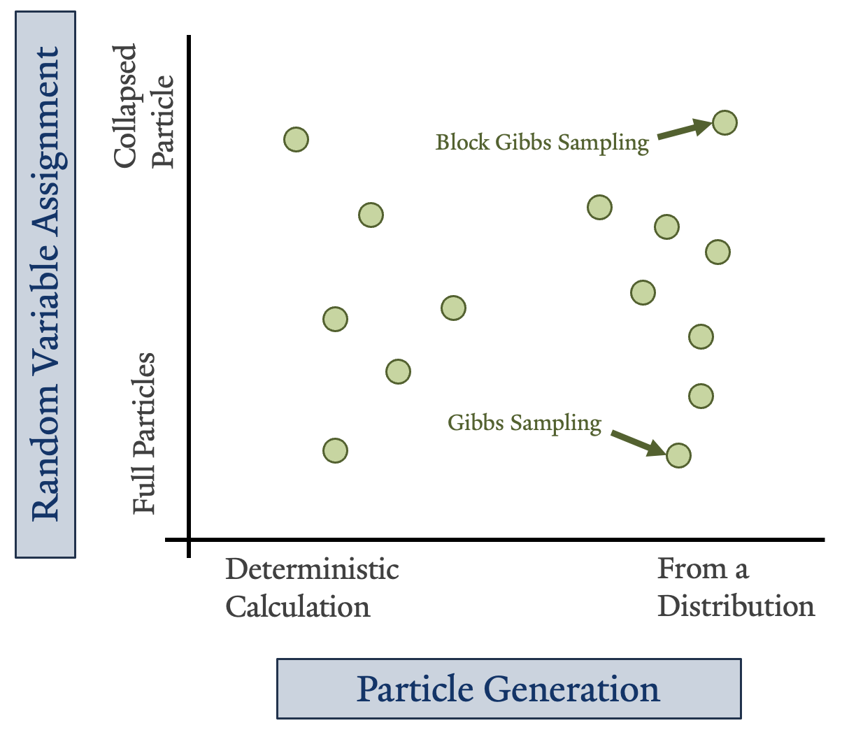
Particle-based methods approximate a multivariate distribution or network with a set of instantiations, referred to as particles, of some or all of the random variables in that distribution2. There are different flavors of this type of method illustrated on the right. Some particles are generated directly from an equation, while others are sampled from a distribution. Some particles represent all the variables in a distribution or network individually, while others assign a proxy variable that groups them 2.
Today we are discussing one type of particle estimation: Gibbs sampling. In most cases, random variables are represented individually. However, readers should be aware that there are variations of Gibbs sampling that facilitate grouping the full set of random variables into “blocks”.
This section summarizes relevant concepts presented in Wasserman’s All of Statistics, specifically Chapter 23 3. Unless otherwise noted, the content comes from Wasserman’s All of Statistics.
A stochastic process \{X_t : t \in T\} is a collection of random variables taken from a state space, \mathcal{X}, and indexed by an ordered set T, which can be interpreted as time. The index set T can be discrete, such as T = \{0, 1, 2, \dots\}, or continuous, such as T = [0, \infty). To denote the stochastic nature of X, it can be written as X_t or X(t).
A Markov chain is a type of stochastic process where the distribution of future states depends only on the current state and not on the sequence of events that preceded it. For example, the outcome for X_t depends only on what the outcome was for X_{t-1}. Notice that sometimes, authors will specify that X is a Markov chain stochastic process by writing X_n instead of X_t.
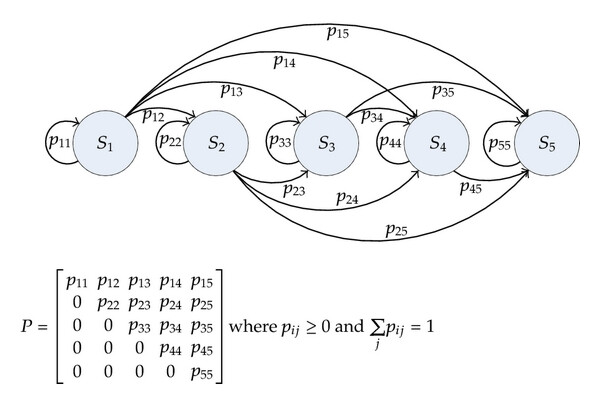
The figure on the left shows a state transition diagram for a discrete-time Markov chain with transition probabilities p_{ij} = \mathbb{P}(X_{n+1}= j\ \lvert\ X_n = i). Below the diagram is the matrix representation of these interactions, known as the transition matrix, \mathbf{P}, where each row is a probability mass function. A generalized definition for a Markov chain is given by
\mathbb{P}(X_n = x\ \lvert\ X_0, \dots, X_{n-1}) = \mathbb{P}(X_n = x\ \lvert\ X_{n-1})
for all n and for all x \in \mathcal{X}. Markov chains have many aspects, but for this application, it is essential to consider the properties of a specific transitional stage denoted by, \pi = (\pi_i : i \in \mathcal{X}). The vector \pi consists of non-negative numbers that sum to one and is a stationary (or invariant) distribution if \pi = \pi\mathbf{P}.
By applying the Chapman-Kolmogorov equations for n-step probabilities, where it is shown that p_{ij}(m+n) = \sum_k p_{ik}(m) p_{kj}(n), we derive that a key characteristic of a stationary distribution \pi for a Markov chain is that it is limiting. This means that, after any number of steps n, a distribution that reaches \pi remains as \pi:
Draw X_0 from the distribution \pi gives \mu_0 = \pi.
Draw X_1 from the distribution \pi gives \mu_1 = \mu_0\mathbf{P} = \pi\mathbf{P} = \pi.
Draw X_2 from the distribution \pi gives \pi\mathbf{P}^2 = (\pi\mathbf{P})\mathbf{P} = \pi\mathbf{P} = \pi.
\dots etc.
Here, \mu_n(i) = \mathbb{P}(X_n = i) denotes the marginal probability that the chain is in state i at time n, while \mu_0 represents the initial distribution. Once the chain limits to the distribution \pi, it will remain in this distribution indefinitely. However, ensuring the process is stationary is not sufficient; it is also important to guarantee that \pi is unique. This uniqueness is guaranteed if the Markov chain is ergodic, which must satisfy the following two characteristics 3,7:
If the Markov chain is also irreducible, then all states communicate, meaning it is possible to get from any state to any other state, denoted by i \leftrightarrow j. Having an irreducible, ergodic Markov chain guarantees that it has a unique stationary distribution, \pi.
A Markov chain with a stationary distribution does not mean that it converges.
There is much more to learn about Markov chains beyond what was discussed here, but these fundamental concepts provide a foundation for understanding their use in Monte Carlo methods.
Traditionally, Monte Carlo methods rely on independent sampling. However, MCMC methods rely on a dependent Markov sequence with a limiting distribution that corresponds to the distribution we aim to model 1. MCMC has wide-ranging applications and is frequently used in Bayesian inference. However, it is also generalizable to other problems that are not Bayesian in nature 1.
To help you understand the connection between Monte Carlo sampling methods and estimating complex analytical solutions using Markov chains, let’s first explore the motivation: initially within the commonly exemplified Bayesian framework, and then in a general sense. Consider the following scenario provided by Wasserman in the context of Bayesian inference where we have a process that generates the random vector X 3. We have the prior distribution f(\theta) with respect to parameter \theta and data \mathbf{X} = (X_1, \dots, X_n) with a posterior density
f(\theta\ \lvert\ \mathbf{X}) = \frac{\mathcal{L}(\theta)\ f(\theta)}{\int \mathcal{L}(\theta)\ f(\theta)\ d\theta}
where the denominator is the normalizing constant, here denoted by c. The mean of the posterior is \begin{align*} \bar{\theta} &= \int \theta\ f(\theta\ \lvert\ \mathbf{X})\ d\theta \\ &= \frac{1}{c} \int \theta\ \mathcal{L}(\theta)\ f(\theta)\ d\theta \end{align*}
If the parameter space is multidimensional, i.e., \boldsymbol{\theta} = (\theta_1, \dots, \theta_k), but we are only interested in one component, say \theta_1, then the marginal posterior density of \theta_1 is defined as f(\theta_1\ \lvert\ \mathbf{X}) = \int\int\cdots\int f(\theta_1, \dots, \theta_k\ \lvert\ \mathbf{X})\ d\theta_2 \cdots\ d\theta_k
As can easily be seen, it might not always be feasible to calculate this outcome directly. Generally speaking, we have a random vector \mathbf{X} and we wish to compute E[f(\mathbf{X})] 1. If the random vector is continuous and associated with the probability density p(\boldsymbol{x}), then we want to calculate E[f(\mathbf{X})] = \int f(\boldsymbol{x})\ p(\boldsymbol{x})\ d\boldsymbol{x}
The density p(\boldsymbol{x}) is often referred to as the target density, representing the distribution of the random variables that are of interest in our study 1.
Markov chains are typically reserved for discrete outcomes. However, general applications of MCMC can be used for discrete, continuous, or hybrid outcomes. In this context, Markov chains can be applied to any type of distribution 1.
Standard Monte Carlo methods aim to draw n independent, identically distributed (i.i.d.) samples of \mathbf{X} directly from p(\boldsymbol{x}), but this is also not always feasible 1. Simple random generation methods require specific restrictions to ensure a solution or might be computationally inefficient in high-dimensional problems. For example, the adaptation of the accept-reject method from Monte Carlo Statistical Methods by Robert and Casella, called adaptive rejection sampling, is restricted to densities that are log-concave and has computational power requirements that are proportional to the fifth power of \text{dim}(\mathbf{X}) 1,8.
Canonical Monte Carlo approaches are more restrictive than is necessary to estimate E[f(\mathbf{X})]. Leveraging Markov chain-based schemes avoids the necessity of sampling directly from p(\boldsymbol{x}); instead, dependent sequences with a limiting distribution of p(\boldsymbol{x}) are used 1.
Recall that in the previous section, we showed that a Markov chain that is irreducible and ergodic is guaranteed to have a unique stationary distribution, \pi 3. This is a consequence of the ergodic theorem, which guarantees that the normalized sum below will approach the mean of f(\mathbf{X}), with convergence in mean square (m.s.) or almost surely (a.s.) as n \rightarrow \infty for any fixed M 1.
\frac{1}{n-M} \sum_{k = M+1}^n\ f(\mathbf{X}_k)
Here, M is referred to as the “burn-in” period. We know that the dependence of \mathbf{X}_k on early states, say \mathbf{X}_0, \mathbf{X}_1, \dots, \mathbf{X}_M, for bounded M < \infty, disappears as k \rightarrow \infty 1. With sufficient burn-in, we achieve the ergodic average that stabilizes at \pi, and when executed correctly, \pi equals the target density to within a scalar value 1,3.
This excerpt summarizes Spall’s Introduction to Stochastic Search and Optimization: Estimation, Simulation, and Control Appendix C.2 Convergence Theory 1.
Finite-sampled stochastic algorithms are often intractable, justifying the focus on the behavior of stochastic processes in their limit. The type of convergence properties a process has informs us about the scenarios where it is appropriate to apply the theory in practice and provides insight into non-limiting behaviors. Convergence for stochastic algorithms is probabilistic and characterized by measure-theoretic concepts, often classified into the following four types:
\gdef\norm#1{\left\lVert#1\right\rVert}
Convergence almost surely: The sequence of random vectors \mathbf{X}_k \rightarrow \mathbf{X} a.s. (or with probability 1)
P\left(\omega \in \Omega \ : \ \lim_{k \rightarrow \infty}\ \norm{\mathbf{X}_k(\omega) - \mathbf{X}(\omega)} = 0\right) = 1
Convergence in probability: The sequence of random vectors \mathbf{X}_k \rightarrow \mathbf{X} in pr.
\lim_{k \rightarrow \infty} P\left(\omega \in \Omega \ : \ \norm{\mathbf{X}_k(\omega) - \mathbf{X}(\omega)} \geq c\right) = 0\ \ \ \text{ for any } c > 0
Convergence in mean square: The sequence of random vectors \mathbf{X}_k \rightarrow \mathbf{X} in m.s.
\lim_{k \rightarrow \infty} E\left(\norm{\mathbf{X}_k(\omega) - \mathbf{X}(\omega)}^2\right) = 0
Convergence in distribution: The sequence of random vectors \mathbf{X}_k \rightarrow \mathbf{X} in m.s.
\lim_{k \rightarrow \infty} F_{\mathbf{X}_k}(\boldsymbol{x}) = F_{\mathbf{X}}(\boldsymbol{x})\ \ \ \text{ at every point } \boldsymbol{x} \text{ where } F_{\mathbf{X}}(\boldsymbol{x}) \text{ is continuous.}
where \norm{\cdot} denotes any valid norm, i.e., the Euclidean norm \norm{\boldsymbol{x}} = \sqrt{\sum_i x_i^2}, and x_i is the i^{th} component of the vector \boldsymbol{x}.
In the next section, we will show how Gibbs sampling produces the correct mean, computed with respect to our target density p(\boldsymbol{x}). In summary, we have thus far introduced the basic concepts around Markov chains that simplify random sampling from conditional distributions, which are guaranteed to converge if irreducible and ergodic. With the appropriate burn-in, M, we can ensure the ergodic average stabilizes at \pi. We now want to show that Gibbs sampling is capable of producing a stabilized limiting distribution, \pi, that is proportional to our target density p(\boldsymbol{x}).
The concept of Gibbs sampling was introduced by Geman and Geman in their paper Stochastic Relaxation, Gibbs Distributions, and the Bayesian Restoration of Images 1,7,9. In their work, they identified the equivalence between Markov random fields and the Gibbs distribution, also known as the Boltzmann distribution, which had been previously used in physical chemistry to relate the probability of a system’s state to its energy and temperature 9,10.
Gibbs sampling is named after the American mechanical engineer and scientist, Josiah Willard Gibbs, who received the first Ph.D. in engineering in the United States in 1863 from Yale University. He was also appointed the first chair of mathematical physics in the United States at Yale, and contributed to many areas in physics, chemistry, and mathematics. Gibbs is credited with laying the foundation for the field of physical chemistry 7,11.
Fundamentally, this is why Gibbs sampling has a natural intuition tied to graphical modeling, a broader subject that we will only lightly touch upon in this week’s concept. Some sources attempt to explain Gibbs sampling outside of the graphical model framework, but the more comprehensive ones will acknowledge this connection. It is beyond our scope to bring students entirely up to speed with graphical theory, so additional reading has been provided earlier to help bridge this gap if readers find any of the content too advanced.
In practice, especially in medical diagnosis problems, there may be hundreds of attributes that contribute to the joint probability distribution for a given disease 2. Furthermore, some of these distributions may overlap or have similarities with those of other diseases, making them challenging to separate using standard probabilistic approaches. Probabilistic graphical models are graph-based representations of variable interactions, which can help to succinctly represent these interactions in digestible pieces despite their high dimensionality 2.
More impressively, graphical modeling encodes interaction attributes such as independencies, factorization, pathways, and message propagation. This not only provides an intuitive understanding of complex interactions but also allows for the exploitation of these features for inference and efficient computation 2,7. Shown below are two fundamental ways in which variables and their relationships with one another can be represented: a Bayesian network, also referred to as a Directed Graph, and a Markov network, also known as an Undirected Graph.
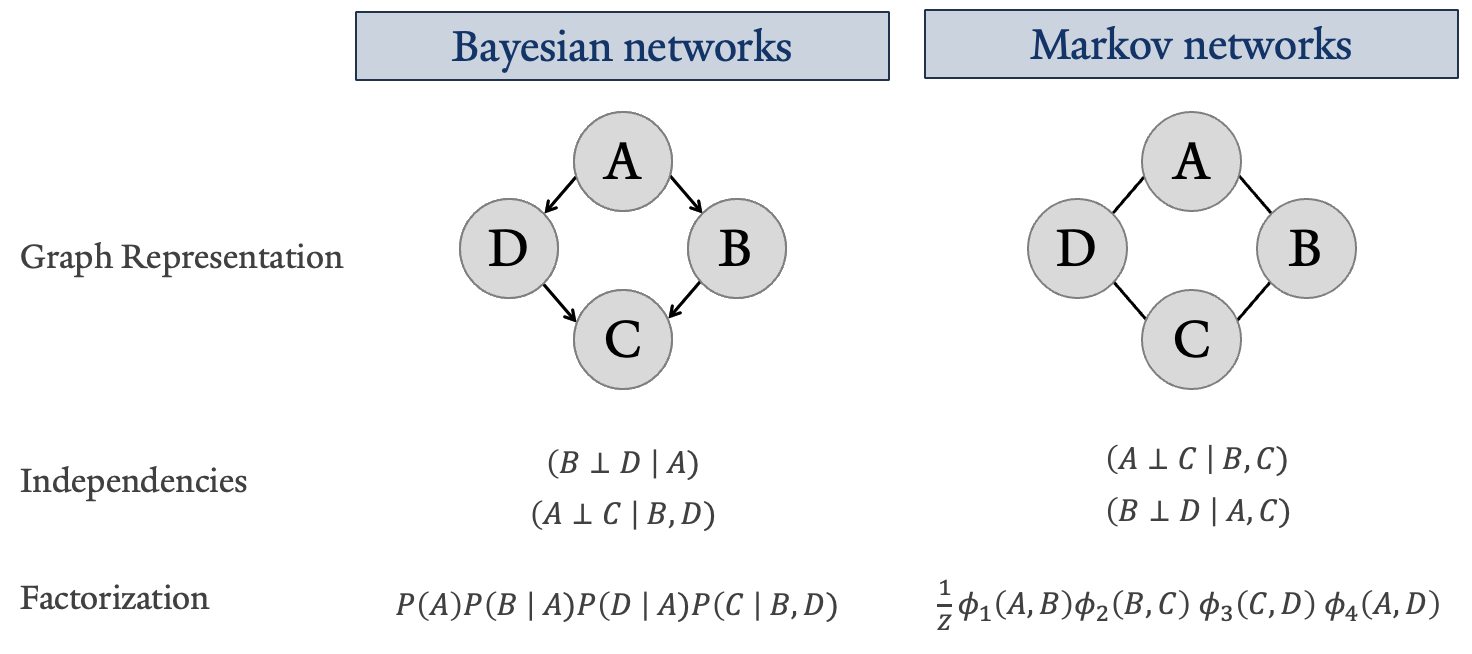
The key concept exemplified by the figure above is independence properties. These can differ for the same graph depending on whether the relationships between variables are defined as directed or undirected, but ultimately allow for factorization representing these independence assertions. The notation differences for factorized joint distributions, shown at the bottom of the figure, are used to differentiate the types of dependency structures implied by the graph itself.
By definition, the Markov network factorization is a Gibbs distribution parameterized by the set of factors \Phi = {\phi(A, B), \phi(B, C), \phi(C, D), \phi(A, D)} with the normalizing constant called the partition function
Z = \sum_{X_1, \dots, X_n}\ \tilde{P}_{\Phi}(X_1, \dots, X_n) where \tilde{P}_{\Phi} represents the joint distribution factorized into conditional probabilities based on its independencies 2.
A factor is one contribution to the overall joint distribution, while a marginal represents a distribution where at least one variable from the joint has been summed or integrated out 2.
Although we have discussed Markov chains earlier and provided the explicit definition of a Gibbs distribution in the context of probabilistic graphical modeling, this does not imply that Gibbs sampling is exclusively applicable to undirected graphs 7. How the differences affect Gibbs sampling is discussed in the next section.
In the M-H algorithm, we start with a proposed distribution, q(\cdot\ \lvert x), from which we can sample, but which is not directly the target distribution, p(\boldsymbol{x}). In many cases, it may be chosen arbitrarily, as long as its limiting behaviors converge to the target distribution 1. For MCMC conducted using the M-H algorithm to work, we need to ensure \pi satisfies detailed balance, where the probability of transitioning from state i to j must be equal to the probability of the reverse transition when multiplied by their respective stationary distribution probabilities 3.
\pi_i p_{ij} = \pi_j p_{ji}
At each step in the algorithm, a candidate point is drawn from the proposal distribution, denoted using the random variable \mathbf{W}. Assuming that this proposal distribution satisfies detailed balance and is a superset of the points for the target distribution (ensuring they are fully supported), then candidate draws are kept or discarded with probability \rho(\mathbf{X}_k, \mathbf{W}) 1
\rho(\boldsymbol{x}, \boldsymbol{w}) = \min\left\{\frac{p(\boldsymbol{w})}{p(\boldsymbol{x})} \frac{q(\boldsymbol{x}\ \lvert\ \boldsymbol{w})}{q(\boldsymbol{w}\ \lvert\ \boldsymbol{x})},\ 1\right\}
If a candidate point is accepted, then \mathbf{X}_{k+1} = \mathbf{W}; otherwise, \mathbf{X}_{k+1} = \mathbf{X}_k 1.
When samples from the Markov chain start to resemble the target distribution, it is said to be “mixing well” 3. Tweaking the parameters used in the proposed distribution to support good mixing is not always straightforward and may require some trial-and-error troubleshooting; refer to example 24.10 from Wasserman’s All of Statistics for an illustration of this.
Gibbs sampling is much like M-H, but it is a special case where the proposal distribution comes directly from the conditional factorizations of p(\boldsymbol{x}) itself. In a sense, it can be thought of as m M-H algorithms working together, where each proposed distribution is one conditional factorization of p(\boldsymbol{x}) 1. In this context, m represents the number of random variables, each having its own conditional distribution for sampling. Consider the following scenario from Spall where we have a distribution p_{X,Y,Z}(\cdot) that we wish to sample from:
At the end of this process, you will have produced the Gibbs sequence. For the example above, we produce:
Y_0, Z_0;\ X_1, Y_1, Z_1;\ X_2, Y_2, Z_2;\ \dots; X_n, Y_n, Z_n
The process described above is iterated over all variables and conditional statements until it is possible to compute the ergodic average. According to the ergodic theorem, this occurs when a sufficient burn-in period has been allowed to run. Using the example above, if we set our burn-in period to M < n, then the appended Gibbs sequence {X_{M+1}, Y_{M+1}, Z_{M+1}; \dots; X_n, Y_n, Z_n} represents measurements that converge in distribution as n \rightarrow \infty to the unique, stationary distribution \pi, that is p_{X,Y,Z}(\cdot) 1.
Finally, the Gibbs sequence results considering the burn-in are substituded into the following equation to give E[f(X,Y,Z)]
\frac{1}{n-M} \sum_{k = M+1}^n\ f(\mathbf{X}_k)
Notice that samplings for X, Y, and Z will converge to their respective marginal distributions, p_X(x), p_Y(y), and p_Z(z); see Section 7.1.3 from Monte Carlo Statistical Methods by Robert and Casella 1,8.
The procedure we have detailed here to estimate the distribution using the collected Gibbs sequence is one of several methods. As might be expected, successive samples drawn from the Markov chain are highly correlated with one another 7. Different approaches are applied if it is desirable to make the values more i.i.d. You can learn more about some of these techniques in Introduction to Stochastic Search and Optimization: Estimation, Simulation, and Control, Section 16.3 Gibbs Sampling by Spall 1.
Because we are drawing from the conditioned factors of the target distribution, this makes Gibbs sampling less generalizable than M-H, but it comes with advantageous trade-offs. For instance, drawing directly from the target distribution itself ensures that detailed balance is already satisfied, and the algorithm is expected to be more efficient because the new point is always accepted 1,2,7.
It is helpful to see the process illustrated for a simpler case, but for completeness, it’s important to know how this extends to a generalized representation. The following is the generalized definition provided by Spall 1. Say that \mathbf{X} is a collection of m univariate components, then the k^{th} sample from X using the previous algorithm is
\mathbf{X}_k = \left[ \begin{array}{c} X_{k1} \\ X_{k2} \\ \vdots \\ X_{km} \end{array} \right]
where X_{ki} is the i^{th} component for the k^{th} replicate of \mathbf{X} that was generated using Gibbs sampling. Denote the step-wise updating results that have been conditioned on the previous samples by \{X_{k+1,\ i}\ \lvert\ \mathbf{X}_{k\backslash i}\} where
\mathbf{X}_{k\backslash i}\ \equiv \{X_{k+1,\ 1},\ X_{k+1,\ 2}, \dots, X_{k+1,\ i-1},\ X_{k,\ i+1} \dots,\ X_{k,\ km}\}
for i = 1,\ 2, \dots,\ m. Use \{X_{k+1,\ i} \mid \mathbf{X}_{k\backslash i}\} \sim p_i(x \mid \mathbf{X}_{k\backslash i}) to represent the sampling density for that random variable conditioned on the current elements of the Gibbs sequence, where i-1 elements are sample points at iteration k+1 and the remaining m-i elements are from the k^{th} iteration. The Gibbs sampling algorithm is as follows:
(Initialization) Choose the length of the burn-in, M, and some arbitrary initial state \mathbf{X}_0 with k=0.
Generate \mathbf{X}_{k+1} by recursively updating the conditionals for each new sampling of a given variable.
\vdots
Repeat step 2 until the burn-in is reached. Set \mathbf{X}_k = \mathbf{X}_M and continue with the procedure laid out in step 2, storing or recursively averaging the results as they are sampled.
When it is possible to compute the ergodic average (i.e. sufficient convergence is observed), then estimate E[f(\mathbf{X})] for the target distribution p(\cdot).
We are only focusing on the typical case where X_{ki} is scalar (i.e., all components of X are univariate). It is sometimes applicable to make them multivariate. Students who wish to explore this further are encouraged to review example 16.7 Variance-components model from Section 16.6 Applications in Bayesian Analysis in Spall’s Introduction to Stochastic Search and Optimization: Estimation, Simulation, and Control 1.
When sampling from the conditional distribution is challenging or requires excessive computational power, the conditional properties associated with a distribution network graph can help 2. Depending on the type of associations defined, it might be possible to isolate variables from the rest of the network using its independence structures, assuming that these assertions are reasonably correct.
For an undirected Markov network, this would involve isolating nodes contained within a Markov blanket. In directed graphs, nodes conditioned on their parents can lead to log-concave Gibbs sampling distributions. If these conditional distributions are log-concave, alternative sampling methods, such as the aforementioned adaptive rejection sampling method, can be used within the Gibbs sampling framework 7,8.
With this fundamental understanding of Gibbs sampling of Markov chains, we are now better prepared to explore hierarchical modeling of our data.
The goal of this exercise is not to comprehensively teach you hierarchical modeling concepts in a way that enables you to derive your own models. Instead, it is intended to introduce you to the concept of breaking down complex systems of interactions into interrelated hierarchies or multilevel distributions. This section aims to introduce enough related concepts to help you follow the example below, interpret the results, and effectively apply the knowledge to your own study. For additional reading on the subject, please refer to the textbooks listed earlier.
Hierarchical models, also known as multilevel models, equip us with the ability to separate features of our set of random variables into layers, contextualizing information that would otherwise not be accounted for in a single distribution. This can occur either methodologically, where units of analysis come from strongly dependent clusters, or substantively, where a predictors influence on a model may vary depending on the context 5.
It is a versatile tool designed to address various inferential goals, including causal inference, prediction, and descriptive modeling. Such models are especially effective for capturing the intricacies of social science or biological processes, which are characterized by complex, interdependent, and situationally interconnected components 4.
To start developing an intuition for hierarchical modeling, it is helpful to work through a simplified example in detail. Consider the following Binomial-Poisson hierarchy example from Statistical Inference by Casella and Berger (example 4.4.1) 12.
We aim to model the survival probability of eggs laid by an insect and estimate the average number expected to survive. For a single insect, the number of eggs laid can be represented using two models:
This setup leads to the following hierarchical model:
\begin{align*} X \lvert Y &\sim \text{binomial}(Y, p)\\ Y &\sim \text{Poisson}(\lambda) \end{align*}
In this example, it is possible to estimate the expectation of X = number of survivors deterministically 12,13.
\begin{align*} P(X = x) &= \sum_{y=0}^{\infty} P(X=x,\ Y=y)\\ &= \sum_{y=0}^{\infty} P(X=x\ \lvert Y=y) P(Y=y)\hspace{45mm} \tag{by definition of $P(X \lvert Y)$}\\ &= \sum_{y=x}^{\infty}\ \left[\binom{y}{x}\ p^x(1-p)^{y-x}\right]\ \left[\frac{e^{-\lambda}\lambda^y}{y!}\right] \tag{$P(X \lvert Y)=0$ when $y<x$}\\ &= \frac{(\lambda p)^x e^{-\lambda}}{x!}\ \sum_{y=x}^{\infty}\ \frac{((1-p)\lambda)^{y-x}}{(y-x)!} \tag{multiply by $\lambda^x/\lambda^x$}\\ &= \frac{(\lambda p)^x e^{-\lambda}}{x!}\ \sum_{t=0}^{\infty}\ \frac{((1-p)\lambda)^{t}}{(y-x)!} \tag{set $t=y-x$}\\ &= \frac{(\lambda p)^x e^{-\lambda}}{x!}\ e^{(1-p)\lambda} \tag{sum of a power series is exponential}\\ &= \frac{(\lambda p)^x e^{-\lambda p}}{x!} \end{align*}
giving us X \sim \text{Poisson}(\lambda p). Using the definition of the first moment of a Poisson distribution we get E(X) = \lambda p. This gives rise to the following theorem from Statistical Inference by Casella and Berger 12:
Theorem 4.4.3 Provided the expectations exist, if X and Y are any two random variables, then E(X) = E(E(X\ \lvert\ Y))
A hierarchy is not confined to two stages; however, it is theoretically possible to simplify some multilevel hierarchies into a two-stage structure 12. Consider the following generalization of the previous example from Statistical Inference by Casella and Berger (example 4.4.5) 12.
Let’s say we want to account for variation between insect mothers, where one is chosen at random for modeling expected survival outcomes of the eggs. We now represent our hierarchical model with the following three equations:
\begin{align*} X \lvert Y &\sim \text{binomial}(Y, p)\\ Y \lvert \Lambda &\sim \text{Poisson}(\Lambda)\\ \Lambda &\sim \text{exponential}(\beta) \end{align*}
where \Lambda is the probability of choosing any given insect mother. Using theorem 4.4.3 we get the mean of X to be:
\begin{align*} E(X) &= E(E(X \lvert Y))\\ &= E(pY)\\ &= E(E(pY \lvert \Lambda))\\ &= E(p\Lambda)\\ &= p\beta \tag{exponential expectation} \end{align*}
As previously mentioned, it is sometimes possible to reduce models with more than two stages to a two-stage setup. In our current example, we can deterministically derive a combined distribution for Y using the related stages Y \lvert \Lambda \sim \text{Poisson}(\Lambda) and \Lambda \sim \text{exponential}(\beta) 12,14.
\begin{align*} P(Y = y) &= P(Y = y, 0 < \Lambda < \infty)\\ &= \int_0^{\infty}\ f(y, \lambda)\ d\lambda\\ &= \int_0^{\infty}\ f(y\ \lvert\ \lambda)\ f(\lambda)\ d\lambda\\ &= \int_0^{\infty}\ \left[\frac{e^{-\lambda}\lambda^y}{y!}\right]\ \frac{1}{\beta}e^{-\lambda/\beta}\ d\lambda\\ &= \frac{1}{\beta y!}\ \int_0^{\infty}\ \lambda^y\ e^{-\lambda\left(1+\beta^{-1}\right)}\ d\lambda\\ &= \frac{1}{\beta y!}\ \left(\frac{1}{1+\beta^{-1}}\right)^{y+1}\ \Gamma(y+1) \tag{gamma PDF kernel}\\ &= \frac{1}{\beta}\ \frac{\beta}{\beta+1} \left(\frac{1}{1+\beta^{-1}}\right)^{y} \tag{$\Gamma(y+1) = y!$}\\ &= \frac{1}{\beta+1} \left(\frac{1}{1+\beta^{-1}}\right)^{y} \end{align*}
which is the negative binomial distribution with p = 1/(\beta + 1) and r = 1. Therefore, our three-stage hierarchical model can be simplified to:
\begin{align*} X \lvert Y &\sim \text{binomial}(Y, p)\\ Y &\sim \text{NB}\left(\frac{1}{\beta+1},\ 1\right) \end{align*}
This is a specific case of the Poisson-gamma mixture, with \Lambda \sim \text{gamma}(\alpha, \beta), which results in a negative binomial marginal distribution for Y.
Although the gamma function extends to complex numbers, we will restrict its definition to real, strictly positive integers, b, (i.e., \mathbb{R}(b) > 0). In this form, the gamma function can be defined as follows 12,15:
\Gamma(b + 1) = \int_0^{\infty}\ t^{b}e^{-t}\ dt
It is common to encounter the expression f(t)e^{g(t)}, which can sometimes be solved using the gamma function with a simple change of variables where u := g(t), such as in our context above. Here we see that g(\lambda) = a\lambda = \lambda\left(1+\beta^{-1}\right), therefore we set our variable substitution to u = \lambda\left(1+\beta^{-1}\right). To make the change of variables coencide with a gamma function, we multiply the integrand by \left(1+\beta^{-1}\right)^{y+1}/\left(1+\beta^{-1}\right)^{y+1}
\left[\int_0^{\infty}\ \lambda^{y}\ e^{-\lambda\left(1+\beta^{-1}\right)}\ d\lambda\right] \frac{\left(1+\beta^{-1}\right)^{y+1}}{\left(1+\beta^{-1}\right)^{y+1}} = \frac{\left(1+\beta^{-1}\right)}{\left(1+\beta^{-1}\right)^{y+1}}\ \int_0^{\infty}\ \left(\lambda\left(1+\beta^{-1}\right)\right)^{y}\ e^{-\lambda(1 + \beta^{-1})}\ d\lambda
set u = \lambda\left(1+\beta^{-1}\right) and du = \left(1+\beta^{-1}\right)\ d\lambda
\begin{align*} &= \frac{\left(1+\beta^{-1}\right)}{\left(1+\beta^{-1}\right)^{y+1}}\ \int_0^{\infty}\ \frac{u^y\ e^{-y}}{\left(1+\beta^{-1}\right)}\ du\\ &= \frac{1}{\left(1+\beta^{-1}\right)^{y+1}}\ \Gamma(y+1)\hspace{45mm} \tag{by definition of gamma function} \end{align*}
mixture distribution: is typically used to refer to a random variable with a distribution that depends on quantities or parameters that themselves have a distribution. The example presented above is a mixture distribution. Not all higherarchical models need to be mixture distributions.
As you might expect, there is a natural connection between the representation of hierarchical distributions and the graphical representation of these relationships. However, this is not always the case. We must be cautious about how variable interactions are represented graphically, as they imply specific variable interaction behaviors that might not be valid 3.
From Chapter 19.3 Hierarchical Log-Linear Models in Wasserman’s All of Statistics:
19.9 Lemma. A graphical model is hierarchical, but the reverse need not be true.
Gibbs sampling is inherently suited to address multivariate problems because it breaks a high-dimensional vector into lower-dimensional component blocks 1.
The rjags package requires JAGS to be installed separately. rjags will reference the JAGS libjags.4.dylib library file and the modules-4 directory, which contains seven *.so files, such as bugs.so. The next steps will walk you through installation, and an optional troubleshooting guide if R cannot find the JAGS file path.
From JAGS, open the download link that will take you to a SourceForge page.
Download the latest version. At the time of this writing, the current version is JAGS-4.3.2.
Open and run the downloaded installer.
Confirm that the installation is located where we need it to be: /usr/local/lib/.
Command-Line Application
# Running both should NOT give you "No such file or directory"
ls -l /usr/local/lib/libjags.4.dylib
ls -l /usr/local/lib/JAGS/modules-4/Sometimes, the installer might place the JAGS program in a different location. For example, if you installed JAGS using Homebrew, the program might have been placed in the Homebrew library. If the file path differs, you will need to adjust the following code accordingly before reinstalling it in R.
Command-Line Application
# This example assumes that Homebrew was used
brew install jags
Open /usr/local/lib by searching for it with “Go to Folder” in an open Finder Window. If it does not already exist, create the file path using the following code.
Command-Line Application
# ONLY IF there is no existing directory
sudo mkdir -p /usr/local/lib
Create a symbolic link from the Homebrew-installed libjags.4.dylib JAGS library to the expected location:
Command-Line Application
sudo ln -s /opt/homebrew/lib/libjags.4.dylib /usr/local/lib/libjags.4.dylibCreate another symbolic link for the Homebrew-installed JAGS modules directory to the expected location:
Command-Line Application
sudo mkdir -p /usr/local/lib/JAGS/modules-4
sudo ln -s /opt/homebrew/lib/JAGS/modules-4/* /usr/local/lib/JAGS/modules-4/
OPTIONAL: You can verify the linking worked if you see the intended directory listed for both of the following lines of code.
Command-Line Application
# Running both should NOT give you "No such file or directory"
ls -l /usr/local/lib/libjags.4.dylib
ls -l /usr/local/lib/JAGS/modules-4/
Reinstalling rjags with the connection in place.
RStudio
# Remove existing installation
remove.packages("rjags")

# Reinstall rjags
install.packages("rjags")

# Load the package
library(rjags)This page was developed on a Mac, and so the directions for a PC were not able to be tested.
From JAGS, open the download link that will take you to a SourceForge page.
Download the latest version. At the time of this writing, the current version is JAGS-4.3.2.
Open and run the downloaded installer.
You will need to also download the latest version of RTools, which at the time of this writing is RTools 4.5. Add Rtools to your PATH if it is not done automatically.
Command-Line Application
where make   # Should give the result "C:\Rtools\bin\make.exe"
echo %PATH%  # Should give the result "C:\Rtools\bin;C:\Rtools\mingw_64\bin"
If this does not give the expected results, you can set the path:
Command-Line Application
# ONLY IF the PATH for Rtools is incorrect.
setx PATH "%PATH%;C:\Rtools\bin;C:\Rtools\mingw_64\bin"
Confirm that the installation is located where we need it to be: C:\Program Files\JAGS\JAGS-4.x\bin.
Command-Line Application
echo %JAGS_HOME%  # Should say "C:\Program Files\JAGS\JAGS-4.x"
echo %PATH% # Should say "...;C:\Program Files\JAGS\JAGS-4.x\bin;..."Sometimes the installer might place the JAGS program in a different location. If this happens, you can set the file path in the command line application as follows and retry installing the package through R.
Modify the environment variables as needed.
Command-Line Application
setx JAGS_HOME "C:\Program Files\JAGS\JAGS-4.x"
setx PATH "%PATH%;C:\Program Files\JAGS\JAGS-4.x\bin"
OPTIONAL: You can verify the setting worked.
Command-Line Application
echo %JAGS_HOME%  # Should say "C:\Program Files\JAGS\JAGS-4.x"
echo %PATH%       # Should say "...;C:\Program Files\JAGS\JAGS-4.x\bin;..."
Reinstalling rjags with the connection in place.
RStudio
# Remove existing installation
remove.packages("rjags")

# Reinstall rjags
install.packages("rjags")

# Load the package
library(rjags)
With JAGS installed, we can now proceed with the standard process of installing the necessary packages. If you have not done so already, you will need to initialize the project’s renv lockfile to ensure that the same package versions are installed in the project’s local package library.
RStudio
renv::init()      # Initialize the project
renv::restore()   # Download packages and their version saved in the lockfile
RStudio
suppressPackageStartupMessages({
  library("readr")      # For reading in the data
  library("tibble")     # For handling tidyverse tibble data classes
  library("tidyr")      # For tidying data
  library("dplyr")      # For data manipulation
  library("stringr")    # For string manipulation
  library("MASS")       # Functions/datasets for statistical analysis
  library("lubridate")  # For date manipulation
  library("ggplot2")    # For creating static visualizations
  library("viridis")    # For color scales in ggplot2
  library("scales")     # For formatting plots axis
  library("gridExtra")  # Creates multiple grid-based plots
  library("rjags")      # For running JAGS (Just Another Gibbs Sampler) models
  library("coda")       # For analysis of MCMC output from Bayesian models
})


# Function to select "Not In"
'%!in%' <- function(x,y)!('%in%'(x,y))
To demonstrate hierarchical modeling using Gibbs sampling to estimate the distribution, we are going to examine the data and results from Potential Impact of Higher-Valency Pneumococcal Conjugate Vaccines Among Adults in Different Localities in Germany by Ellingson et al 16.
The data comes from surveillance for invasive pneumococcal disease (IPD) conducted by the German National Reference Center for Streptococci (GRNCS), which collects voluntarily reported microbial diagnostic lab results and is expected to account for 50% of all IPD in Germany. Serotyping is done by GNRCS using the samples provided by these laboratories, and incidences are reported as cases per 100,000 using the age-specific population in Germany in 2018 16.
# Read in the cleaned data directly from the instructor's GitHub.
df <- read_csv("https://raw.githubusercontent.com/ysph-dsde/bdsy-phm/refs/heads/main/Data/testDE2.csv")

# Summarize the variable names included in the dataset.
colnames(df)
[1] "...1" "Sequencial.number"
[3] "Study" "Number"
[5] "Inclusion" "DateOfIsolation"
[7] "DateOfBirth" "AgeInYears"
[9] "AgeinMonths" "Postleitzahl.patient"
[11] "Zip" "Federal.state.patient"
[13] "Residence.patient" "Country.patient"
[15] "SeroType" "Strain.identification...Genus"
[17] "Strain.identification...Species" "Pneumonia"
[19] "MD.Amoxicillin" "AmoxicillinSNS"
[21] "MD.Cefotaxime" "CefotaximeSNS"
[23] "MD.Chloramphenicol" "ChloramphenicolSNS"
[25] "MD.Clindamycin" "ClindamycinSNS"
[27] "MD.Erythromycin" "ErythromycinSNS"
[29] "MD.Levofloxacin" "LevofloxaxinSNS"
[31] "MD.Penicillin" "PenicillinSNS"
[33] "MD.Tetracyclin" "TetracyclineSNS"
[35] "MD.Trimetoprim.Sulfamethoxazole" "Sulfamethoxazole.trimethoprimSNS"
[37] "MD.Vancomycin" "VancomycinSNS"
[39] "date" "year"
[41] "month" "epiyr"
[43] "agec" "vt"
[45] "vaxperiod" "zip2"
[47] "indic" The dataset includes a lot of information that is not required for our analysis today. We will, therefore, focus only on the variables used in the hierarchical model itself.
# Summarize aspects and dimentions of our dataset.
glimpse(df[, c(39:42, 45, 8, 15)])
Rows: 17,653
Columns: 7
$ date <date> 2003-01-15, 2003-01-15, 2003-01-15, 2003-01-15, 2003-01-15…
$ year <dbl> 2003, 2003, 2003, 2003, 2003, 2003, 2003, 2003, 2003, 2003,…
$ month <dbl> 1, 1, 1, 1, 1, 1, 1, 1, 1, 1, 1, 1, 1, 1, 1, 1, 1, 1, 1, 1,…
$ epiyr <dbl> 2002, 2002, 2002, 2002, 2002, 2002, 2002, 2002, 2002, 2002,…
$ vaxperiod <dbl> 1, 1, 1, 1, 1, 1, 1, 1, 1, 1, 1, 1, 1, 1, 1, 1, 1, 1, 1, 1,…
$ AgeInYears <dbl> 40, 63, 77, 74, 84, 89, 79, 53, 73, 42, 50, 69, 71, 72, 40,…
$ SeroType <chr> "1", "3", "4", "19F", "14", "7F", "7C", "12F", "4", "4", "5…This paper did not explicitly describe each variable in a “Data Dictionary”. The following was assembled based on the context and methods provided in the paper, other like papers by the same authors, and its supplementary materials 16,17.
date: The date when the events were recorded. It is not clear if this is the date GNRCS received the samples or when they were collected at the participating lab.
year: The year from the date column.
month: The month from the date column.
epiyr: The epidemiological year of the observation (MMWR definition) 18.
vaxperiod: Numerical encoding differentiating years where the PCV vaccine recommendations differed, with approximately a one-year latency time built in. It is not clear what each phase denotes, but based on other papers by the same authors, they appear to mean 17:
vaxperiod = 1 The period before Germany instituted its recommendation for all infants to receive 4 PCV doses in July 2006. The specific formula was not enforced and could either have been the 10-valent or 13-valent PCV. Spans 2001 to 2007.vaxperiod = 2 The period following introduction of PCV in infants in 2006 and before the updated recommendation for infants to receive 2 primary doses and a booster dose. Spans 2007 to 2015.vaxperiod = 3 The period following the updated recommendation in 2015. Spans 2015 to 2018.AgeInYears: The age of the patient from which the same was collected.
SeroType: The serotype of the pathogen identified using capsular swelling with the full antiserum.
SeroType and epiyr.# Aggregate the data by SeroType and epiyr to get the number of cases
# for each combination. The function complete() ensures all combinations
# of SeroType and epiyr are represented in the dataset, even those with
# zero cases.
serotype_year_counts <- df %>%
count(SeroType, epiyr, name = "cases") %>%
complete(SeroType, epiyr, fill = list(cases = 0))
# Convert the categorical variables SeroType and epiyr into numeric IDs
# which are easier to work with in JAGS.
serotype_year_counts <- serotype_year_counts %>%
mutate(sero_id = as.integer(factor(SeroType)),
year_id = as.integer(factor(epiyr)))
# Create the data list that will be input into JAGS.
jdat <- list(
N = nrow(serotype_year_counts),
cases = serotype_year_counts$cases,
sero_id = serotype_year_counts$sero_id,
year_id = serotype_year_counts$year_id,
n_sero = length(unique(serotype_year_counts$sero_id)),
n_year = length(unique(serotype_year_counts$year_id))
)In this scenario
jcode <- "
model {
  for (i in 1:N) {
    cases[i] ~ dpois(lambda[i])
    log(lambda[i]) <- mu[sero_id[i]] + beta[sero_id[i]] * (year_id[i] - mean_year)
  }

  for (s in 1:n_sero) {
    mu[s] ~ dnorm(0, 0.001)
    beta[s] ~ dnorm(0, 0.001)
  }

  mean_year <- (n_year + 1) / 2
}
"source("Model2.R")
mod <- jags.model(textConnection(jcode), data = jdat, n.chains = 2)Compiling model graph
Resolving undeclared variables
Allocating nodes
Graph information:
Observed stochastic nodes: 1577
Unobserved stochastic nodes: 166
Total graph size: 9656
Initializing modelupdate(mod, 1000) # burn-in
samp <- coda.samples(mod, variable.names = c("mu", "beta"), n.iter = 5000)
summary(samp)
Iterations = 2001:7000
Thinning interval = 1
Number of chains = 2
Sample size per chain = 5000

1. Empirical mean and standard deviation for each variable,
   plus standard error of the mean:

               Mean        SD  Naive SE Time-series SE
beta[1]  -8.257e-03  0.006958 6.958e-05      9.046e-05
beta[2]   1.310e-01  0.009281 9.281e-05      1.715e-04
beta[3]   1.374e-01  0.045208 4.521e-04      8.832e-04
beta[4]   8.647e-03  0.096593 9.659e-04      1.249e-03
beta[5]   1.252e-01  0.009666 9.666e-05      1.755e-04
beta[6]   7.577e-02  0.081587 8.159e-04      1.200e-03
beta[7]  -5.682e-02  0.120202 1.202e-03      1.655e-03
beta[8]   1.402e-01  0.042943 4.294e-04      8.764e-04
beta[9]  -9.117e-02  0.153139 1.531e-03      2.515e-03
beta[10]  1.789e-01  0.007998 7.998e-05      1.791e-04
beta[11]  1.051e-01  0.045882 4.588e-04      7.868e-04
beta[12] -4.635e-02  0.007432 7.432e-05      1.022e-04
beta[13]  2.024e-01  0.012534 1.253e-04      3.092e-04
beta[14]  1.428e-01  0.014124 1.412e-04      2.621e-04
beta[15]  1.502e-01  0.019810 1.981e-04      3.856e-04
beta[16]  1.039e-01  0.072167 7.217e-04      1.219e-03
beta[17]  2.028e-01  0.019293 1.929e-04      4.958e-04
beta[18]  4.906e+00  2.695424 2.695e-02      8.641e-01
beta[19]  1.708e-01  0.019860 1.986e-04      4.580e-04
beta[20] -1.848e-01  0.271797 2.718e-03      6.921e-03
beta[21]  1.151e-01  0.036451 3.645e-04      6.459e-04
beta[22]  1.514e-01  0.169920 1.699e-03      3.546e-03
beta[23]  1.207e-02  0.014380 1.438e-04      1.833e-04
beta[24] -1.722e-01  0.171158 1.712e-03      3.945e-03
beta[25]  1.009e-01  0.005900 5.900e-05      9.450e-05
beta[26]  2.624e-01  0.310140 3.101e-03      1.014e-02
beta[27] -3.751e-01  0.376178 3.762e-03      1.908e-02
beta[28]  5.305e-02  0.009889 9.889e-05      1.343e-04
beta[29]  1.558e-01  0.014807 1.481e-04      2.933e-04
beta[30]  2.875e-01  0.078268 7.827e-04      2.790e-03
beta[31]  2.966e-02  0.087751 8.775e-04      1.143e-03
beta[32] -1.798e-01  0.181794 1.818e-03      4.383e-03
beta[33]  1.451e-01  0.006523 6.523e-05      1.269e-04
beta[34]  1.629e-01  0.010742 1.074e-04      2.180e-04
beta[35]  3.638e-01  0.343588 3.436e-03      1.335e-02
beta[36]  2.037e-01  0.012513 1.251e-04      3.148e-04
beta[37] -1.686e-01  0.261744 2.617e-03      5.704e-03
beta[38] -1.961e-02  0.010900 1.090e-04      1.441e-04
beta[39]  9.975e-02  0.105616 1.056e-03      1.768e-03
beta[40]  4.052e-02  0.118965 1.190e-03      1.705e-03
beta[41]  1.515e-01  0.011205 1.120e-04      2.241e-04
beta[42]  1.140e-02  0.117694 1.177e-03      1.551e-03
beta[43] -9.222e-03  0.098721 9.872e-04      1.257e-03
beta[44]  1.166e+00  0.711097 7.111e-03      6.477e-02
beta[45]  3.115e+00  1.598370 1.598e-02      3.472e-01
beta[46]  1.775e-01  0.033563 3.356e-04      7.526e-04
beta[47]  1.945e-01  0.056817 5.682e-04      1.444e-03
beta[48]  9.367e-03  0.066897 6.690e-04      8.798e-04
beta[49]  1.410e-01  0.004122 4.122e-05      7.958e-05
beta[50]  1.735e-01  0.016314 1.631e-04      3.585e-04
beta[51] -1.349e-01  0.057255 5.725e-04      1.045e-03
beta[52] -1.156e-01  0.158524 1.585e-03      2.965e-03
beta[53]  1.337e-01  0.013048 1.305e-04      2.456e-04
beta[54]  1.378e-01  0.023283 2.328e-04      4.428e-04
beta[55]  7.857e-02  0.066172 6.617e-04      1.016e-03
beta[56]  1.903e-01  0.017442 1.744e-04      4.291e-04
beta[57]  4.476e-02  0.057298 5.730e-04      7.522e-04
beta[58]  1.537e-01  0.012929 1.293e-04      2.682e-04
beta[59]  1.640e-01  0.051581 5.158e-04      1.073e-03
beta[60]  1.607e-01  0.015102 1.510e-04      3.171e-04
beta[61] -3.319e-04  0.231136 2.311e-03      3.114e-03
beta[62]  3.399e-03  0.008517 8.517e-05      1.088e-04
beta[63] -5.372e-02  0.044018 4.402e-04      6.502e-04
beta[64]  5.152e-03  0.010941 1.094e-04      1.458e-04
beta[65] -1.163e-01  0.249725 2.497e-03      5.460e-03
beta[66] -2.594e-02  0.014109 1.411e-04      1.749e-04
beta[67] -1.140e-01  0.247208 2.472e-03      4.970e-03
beta[68]  1.266e-01  0.010911 1.091e-04      1.979e-04
beta[69]  1.961e-01  0.110582 1.106e-03      2.755e-03
beta[70]  5.133e-02  0.230772 2.308e-03      3.213e-03
beta[71] -1.773e-01  0.271265 2.713e-03      6.845e-03
beta[72]  6.714e-02  0.153407 1.534e-03      2.542e-03
beta[73]  3.534e-01  0.074084 7.408e-04      3.264e-03
beta[74]  1.188e-01  0.042676 4.268e-04      7.586e-04
beta[75]  2.008e-02  0.005673 5.673e-05      7.237e-05
beta[76]  2.043e-01  0.007410 7.410e-05      1.848e-04
beta[77] -4.682e-02  0.072815 7.281e-04      9.706e-04
beta[78] -4.679e-02  0.073358 7.336e-04      1.062e-03
beta[79]  1.649e-01  0.008042 8.042e-05      1.675e-04
beta[80] -1.601e-03  0.235574 2.356e-03      3.149e-03
beta[81] -3.262e-02  0.011099 1.110e-04      1.458e-04
beta[82]  1.719e-01  0.047389 4.739e-04      1.074e-03
beta[83]  2.720e-01  0.207867 2.079e-03      6.846e-03
mu[1]     3.597e+00  0.038497 3.850e-04      4.955e-04
mu[2]     3.046e+00  0.055218 5.522e-04      1.029e-03
mu[3]    -1.232e-01  0.273905 2.739e-03      5.387e-03
mu[4]    -1.811e+00  0.552768 5.528e-03      8.272e-03
mu[5]     2.962e+00  0.056643 5.664e-04      1.014e-03
mu[6]    -1.417e+00  0.474351 4.744e-03      7.589e-03
mu[7]    -2.266e+00  0.711539 7.115e-03      1.240e-02
mu[8]    -5.275e-03  0.260422 2.604e-03      5.198e-03
mu[9]    -2.899e+00  0.960191 9.602e-03      1.894e-02
mu[10]    3.379e+00  0.049983 4.998e-04      1.108e-03
mu[11]   -1.661e-01  0.270123 2.701e-03      4.580e-03
mu[12]    3.494e+00  0.040990 4.099e-04      5.678e-04
mu[13]    2.439e+00  0.079857 7.986e-04      2.001e-03
mu[14]    2.196e+00  0.085188 8.519e-04      1.613e-03
mu[15]    1.532e+00  0.120139 1.201e-03      2.428e-03
mu[16]   -1.144e+00  0.428956 4.290e-03      7.629e-03
mu[17]    1.654e+00  0.122645 1.226e-03      3.112e-03
mu[18]   -4.479e+01 24.077216 2.408e-01      7.774e+00
mu[19]    1.564e+00  0.123113 1.231e-03      2.710e-03
mu[20]   -4.568e+00  1.922192 1.922e-02      5.827e-02
mu[21]    3.284e-01  0.213748 2.137e-03      3.809e-03
mu[22]   -3.134e+00  1.108130 1.108e-02      2.599e-02
mu[23]    2.135e+00  0.079575 7.957e-04      1.042e-03
mu[24]   -3.187e+00  1.116507 1.117e-02      2.713e-02
mu[25]    3.946e+00  0.033818 3.382e-04      5.495e-04
mu[26]   -4.920e+00  2.241045 2.241e-02      8.042e-02
mu[27]   -5.595e+00  2.893082 2.893e-02      1.558e-01
mu[28]    2.911e+00  0.054702 5.470e-04      7.465e-04
mu[29]    2.127e+00  0.090430 9.043e-04      1.820e-03
mu[30]   -1.260e+00  0.541019 5.410e-03      1.944e-02
mu[31]   -1.558e+00  0.494553 4.946e-03      7.304e-03
mu[32]   -3.244e+00  1.209520 1.210e-02      3.229e-02
mu[33]    3.799e+00  0.038853 3.885e-04      7.985e-04
mu[34]    2.782e+00  0.065304 6.530e-04      1.404e-03
mu[35]   -5.492e+00  2.584125 2.584e-02      1.064e-01
mu[36]    2.459e+00  0.080186 8.019e-04      2.020e-03
mu[37]   -4.442e+00  1.748421 1.748e-02      4.505e-02
mu[38]    2.641e+00  0.061073 6.107e-04      7.875e-04
mu[39]   -1.969e+00  0.631656 6.317e-03      1.125e-02
mu[40]   -2.244e+00  0.705906 7.059e-03      1.248e-02
mu[41]    2.680e+00  0.068384 6.838e-04      1.361e-03
mu[42]   -2.215e+00  0.689549 6.895e-03      1.079e-02
mu[43]   -1.827e+00  0.560018 5.600e-03      8.102e-03
mu[44]   -1.168e+01  6.019880 6.020e-02      5.796e-01
mu[45]   -2.870e+01 14.235215 1.424e-01      3.093e+00
mu[46]    4.893e-01  0.210372 2.104e-03      4.673e-03
mu[47]   -5.663e-01  0.362331 3.623e-03      9.309e-03
mu[48]   -1.000e+00  0.383650 3.837e-03      5.417e-03
mu[49]    4.708e+00  0.025094 2.509e-04      4.877e-04
mu[50]    1.928e+00  0.101569 1.016e-03      2.234e-03
mu[51]   -6.424e-01  0.347678 3.477e-03      6.726e-03
mu[52]   -2.983e+00  1.007665 1.008e-02      2.118e-02
mu[53]    2.383e+00  0.077374 7.737e-04      1.428e-03
mu[54]    1.203e+00  0.140149 1.401e-03      2.632e-03
mu[55]   -9.561e-01  0.384277 3.843e-03      6.177e-03
mu[56]    1.834e+00  0.109899 1.099e-03      2.708e-03
mu[57]   -6.688e-01  0.319979 3.200e-03      4.640e-03
mu[58]    2.373e+00  0.079585 7.958e-04      1.626e-03
mu[59]   -4.279e-01  0.318654 3.187e-03      6.843e-03
mu[60]    2.093e+00  0.092620 9.262e-04      1.960e-03
mu[61]   -4.094e+00  1.469400 1.469e-02      2.923e-02
mu[62]    3.202e+00  0.045611 4.561e-04      5.671e-04
mu[63]   -1.008e-01  0.248194 2.482e-03      3.573e-03
mu[64]    2.664e+00  0.060865 6.086e-04      7.970e-04
mu[65]   -4.323e+00  1.683750 1.684e-02      3.992e-02
mu[66]    2.120e+00  0.079974 7.997e-04      9.972e-04
mu[67]   -4.271e+00  1.683477 1.683e-02      4.013e-02
mu[68]    2.728e+00  0.064628 6.463e-04      1.156e-03
mu[69]   -2.051e+00  0.724357 7.244e-03      1.913e-02
mu[70]   -4.100e+00  1.475845 1.476e-02      2.935e-02
mu[71]   -4.527e+00  1.903808 1.904e-02      5.594e-02
mu[72]   -2.862e+00  0.942228 9.422e-03      1.699e-02
mu[73]   -1.295e+00  0.534726 5.347e-03      2.401e-02
mu[74]   -1.090e-02  0.248633 2.486e-03      4.512e-03
mu[75]    3.988e+00  0.030829 3.083e-04      3.927e-04
mu[76]    3.484e+00  0.047774 4.777e-04      1.192e-03
mu[77]   -1.174e+00  0.413566 4.136e-03      5.933e-03
mu[78]   -1.185e+00  0.418433 4.184e-03      6.388e-03
mu[79]    3.322e+00  0.049550 4.955e-04      1.068e-03
mu[80]   -4.143e+00  1.539104 1.539e-02      3.172e-02
mu[81]    2.650e+00  0.062552 6.255e-04      8.574e-04
mu[82]   -2.166e-01  0.295130 2.951e-03      6.788e-03
mu[83]   -3.680e+00  1.464204 1.464e-02      5.038e-02

2. Quantiles for each variable:

               2.5%        25%        50%        75%     97.5%
beta[1]   -0.021963  -0.012811  -0.008259 -3.652e-03  0.005787
beta[2]    0.112776   0.124698   0.130978  1.372e-01  0.149674
beta[3]    0.052655   0.106546   0.135900  1.670e-01  0.229633
beta[4]   -0.181163  -0.055251   0.008160  7.134e-02  0.206079
beta[5]    0.106389   0.118710   0.125169  1.317e-01  0.144879
beta[6]   -0.077566   0.019615   0.072963  1.286e-01  0.242921
beta[7]   -0.300748  -0.132654  -0.052733  2.249e-02  0.172505
beta[8]    0.061474   0.111122   0.139098  1.672e-01  0.229306
beta[9]   -0.415555  -0.186655  -0.084294  1.164e-02  0.193529
beta[10]   0.163350   0.173253   0.178900  1.843e-01  0.194307
beta[11]   0.018292   0.074188   0.103919  1.349e-01  0.198649
beta[12]  -0.060707  -0.051412  -0.046267 -4.124e-02 -0.031998
beta[13]   0.178352   0.193953   0.202020  2.105e-01  0.227793
beta[14]   0.115203   0.133256   0.142637  1.521e-01  0.170519
beta[15]   0.112089   0.136644   0.149916  1.636e-01  0.189827
beta[16]  -0.030150   0.054313   0.100306  1.495e-01  0.253500
beta[17]   0.166512   0.189732   0.202491  2.155e-01  0.242359
beta[18]   0.403496   2.733174   5.032793  6.923e+00  9.975432
beta[19]   0.132643   0.157449   0.170537  1.842e-01  0.210047
beta[20]  -0.826641  -0.329915  -0.157097 -6.915e-03  0.276319
beta[21]   0.046650   0.090004   0.114307  1.389e-01  0.190274
beta[22]  -0.146903   0.035882   0.137084  2.530e-01  0.524007
beta[23]  -0.016066   0.002112   0.012151  2.193e-02  0.039341
beta[24]  -0.545077  -0.278018  -0.158235 -5.421e-02  0.125818
beta[25]   0.089050   0.096948   0.100913  1.048e-01  0.112465
beta[26]  -0.222541   0.053389   0.216160  4.215e-01  0.996707
beta[27]  -1.298808  -0.553031  -0.308675 -1.231e-01  0.157721
beta[28]   0.033821   0.046340   0.053112  5.980e-02  0.072245
beta[29]   0.127625   0.145782   0.155797  1.657e-01  0.184805
beta[30]   0.151548   0.231290   0.280133  3.372e-01  0.456115
beta[31]  -0.142403  -0.028858   0.028459  8.593e-02  0.211344
beta[32]  -0.590480  -0.281068  -0.162461 -5.860e-02  0.132000
beta[33]   0.132689   0.140716   0.145030  1.494e-01  0.158385
beta[34]   0.142338   0.155659   0.162803  1.701e-01  0.184279
beta[35]  -0.168826   0.125089   0.315764  5.483e-01  1.159127
beta[36]   0.179718   0.195252   0.203665  2.121e-01  0.227864
beta[37]  -0.749247  -0.314493  -0.144057  3.612e-03  0.299236
beta[38]  -0.040894  -0.027190  -0.019606 -1.221e-02  0.001877
beta[39]  -0.098521   0.030132   0.096039  1.665e-01  0.318872
beta[40]  -0.188402  -0.038362   0.038571  1.165e-01  0.282323
beta[41]   0.129764   0.143849   0.151359  1.589e-01  0.174409
beta[42]  -0.218930  -0.067007   0.011521  8.770e-02  0.244022
beta[43]  -0.203651  -0.073049  -0.009235  5.458e-02  0.184364
beta[44]   0.060152   0.608523   1.077893  1.637e+00  2.682420
beta[45]   0.539714   1.861771   2.897139  4.187e+00  6.517252
beta[46]   0.115122   0.154064   0.176974  2.000e-01  0.246666
beta[47]   0.091326   0.156065   0.191213  2.304e-01  0.314630
beta[48]  -0.120475  -0.034328   0.008796  5.326e-02  0.141619
beta[49]   0.132758   0.138160   0.140892  1.437e-01  0.149015
beta[50]   0.142220   0.162447   0.173217  1.842e-01  0.207124
beta[51]  -0.251194  -0.172074  -0.133590 -9.567e-02 -0.027211
beta[52]  -0.454042  -0.210566  -0.106215 -1.285e-02  0.174381
beta[53]   0.108591   0.124849   0.133575  1.423e-01  0.159611
beta[54]   0.094146   0.121811   0.137078  1.535e-01  0.185308
beta[55]  -0.049764   0.033901   0.076933  1.222e-01  0.212111
beta[56]   0.156860   0.178254   0.190087  2.018e-01  0.225781
beta[57]  -0.065395   0.006258   0.043595  8.264e-02  0.158565
beta[58]   0.128278   0.144913   0.153656  1.625e-01  0.178958
beta[59]   0.067611   0.127409   0.162173  1.974e-01  0.271309
beta[60]   0.131421   0.150542   0.160543  1.706e-01  0.191098
beta[61]  -0.478360  -0.139081   0.001145  1.440e-01  0.461696
beta[62]  -0.013019  -0.002358   0.003402  9.097e-03  0.020210
beta[63]  -0.140674  -0.083457  -0.052709 -2.415e-02  0.031466
beta[64]  -0.015984  -0.002376   0.005341  1.248e-02  0.026236
beta[65]  -0.672544  -0.258041  -0.097715  4.650e-02  0.331817
beta[66]  -0.053793  -0.035478  -0.026149 -1.654e-02  0.001811
beta[67]  -0.665125  -0.252705  -0.094769  4.527e-02  0.335315
beta[68]   0.105409   0.119155   0.126434  1.341e-01  0.147304
beta[69]   0.002882   0.120106   0.187677  2.642e-01  0.437706
beta[70]  -0.394986  -0.098058   0.045486  1.932e-01  0.530188
beta[71]  -0.812509  -0.321017  -0.148571 -2.057e-04  0.279185
beta[72]  -0.213634  -0.036074   0.059549  1.597e-01  0.394876
beta[73]   0.219106   0.302329   0.349778  4.010e-01  0.510190
beta[74]   0.037882   0.089558   0.118087  1.474e-01  0.204238
beta[75]   0.008893   0.016206   0.020124  2.386e-02  0.031129
beta[76]   0.189891   0.199270   0.204282  2.093e-01  0.219121
beta[77]  -0.191188  -0.094872  -0.045787  1.307e-03  0.093876
beta[78]  -0.192800  -0.094685  -0.044865  3.360e-03  0.094093
beta[79]   0.149270   0.159487   0.164986  1.705e-01  0.180582
beta[80]  -0.473978  -0.146789  -0.003720  1.446e-01  0.469306
beta[81]  -0.054401  -0.040025  -0.032528 -2.514e-02 -0.010736
beta[82]   0.083339   0.138935   0.169975  2.033e-01  0.267733
beta[83]  -0.057314   0.125570   0.246245  3.858e-01  0.759336
mu[1]      3.519641   3.571193   3.597396  3.623e+00  3.672281
mu[2]      2.933617   3.009074   3.047234  3.084e+00  3.150191
mu[3]     -0.703669  -0.292349  -0.107347  6.330e-02  0.365335
mu[4]     -3.023465  -2.147850  -1.761261 -1.422e+00 -0.857178
mu[5]      2.849730   2.923520   2.963091  3.000e+00  3.070461
mu[6]     -2.458618  -1.712910  -1.379806 -1.088e+00 -0.593911
mu[7]     -3.879434  -2.678552  -2.191191 -1.765e+00 -1.096330
mu[8]     -0.560595  -0.169512   0.006274  1.727e-01  0.468983
mu[9]     -5.212282  -3.423714  -2.762758 -2.220e+00 -1.410030
mu[10]     3.279996   3.345843   3.379062  3.413e+00  3.477349
mu[11]    -0.726887  -0.340524  -0.155396  2.298e-02  0.321630
mu[12]     3.412751   3.467144   3.494337  3.522e+00  3.574211
mu[13]     2.276213   2.386411   2.441102  2.493e+00  2.590178
mu[14]     2.025190   2.140280   2.196459  2.254e+00  2.360173
mu[15]     1.289621   1.452643   1.535866  1.613e+00  1.763141
mu[16]    -2.085484  -1.401827  -1.104043 -8.496e-01 -0.395437
mu[17]     1.401370   1.574668   1.657952  1.739e+00  1.879813
mu[18]   -90.629195 -62.754806 -45.625285 -2.536e+01 -5.226556
mu[19]     1.311898   1.482177   1.568300  1.649e+00  1.792317
mu[20]    -9.529609  -5.467108  -4.161041 -3.221e+00 -1.982856
mu[21]    -0.126245   0.194874   0.339332  4.748e-01  0.715101
mu[22]    -5.777991  -3.723475  -2.960127 -2.348e+00 -1.478525
mu[23]     1.974486   2.083011   2.135788  2.190e+00  2.285749
mu[24]    -5.871948  -3.823139  -3.011353 -2.376e+00 -1.492757
mu[25]     3.878226   3.924068   3.946742  3.969e+00  4.010906
mu[26]   -10.544306  -5.943830  -4.421020 -3.345e+00 -1.997753
mu[27]   -13.079475  -6.731291  -4.929606 -3.648e+00 -2.088998
mu[28]     2.804609   2.874158   2.912066  2.949e+00  3.017010
mu[29]     1.944534   2.067580   2.128091  2.189e+00  2.299178
mu[30]    -2.473788  -1.592175  -1.208937 -8.726e-01 -0.352083
mu[31]    -2.620673  -1.861546  -1.524123 -1.207e+00 -0.704217
mu[32]    -6.159054  -3.868904  -3.047151 -2.386e+00 -1.474382
mu[33]     3.721617   3.773088   3.800190  3.826e+00  3.872946
mu[34]     2.650376   2.738882   2.782653  2.826e+00  2.909818
mu[35]   -11.904181  -6.762912  -4.907752 -3.647e+00 -2.168328
mu[36]     2.300372   2.405150   2.460796  2.515e+00  2.611404
mu[37]    -8.546106  -5.342760  -4.107189 -3.200e+00 -1.969897
mu[38]     2.518109   2.600474   2.641097  2.683e+00  2.757249
mu[39]    -3.398537  -2.330494  -1.901776 -1.523e+00 -0.943141
mu[40]    -3.898173  -2.639488  -2.157147 -1.759e+00 -1.091329
mu[41]     2.542746   2.634131   2.681539  2.725e+00  2.810090
mu[42]    -3.763242  -2.636743  -2.139027 -1.724e+00 -1.081648
mu[43]    -3.057359  -2.170065  -1.783567 -1.428e+00 -0.865387
mu[44]   -24.934763 -15.565267 -10.743799 -6.857e+00 -2.947336
mu[45]   -59.161056 -38.219434 -26.774244 -1.749e+01 -6.035742
mu[46]     0.049283   0.352121   0.497663  6.307e-01  0.877714
mu[47]    -1.366754  -0.780286  -0.543486 -3.115e-01  0.057083
mu[48]    -1.812336  -1.246002  -0.977305 -7.282e-01 -0.317618
mu[49]     4.659920   4.691497   4.708481  4.725e+00  4.758529
mu[50]     1.721210   1.863664   1.929059  1.997e+00  2.118982
mu[51]    -1.373095  -0.865179  -0.626792 -3.974e-01 -0.013884
mu[52]    -5.347050  -3.531949  -2.841546 -2.272e+00 -1.451257
mu[53]     2.228896   2.331374   2.383789  2.436e+00  2.531250
mu[54]     0.927755   1.108779   1.205299  1.299e+00  1.468133
mu[55]    -1.784661  -1.195775  -0.931103 -6.833e-01 -0.282734
mu[56]     1.607750   1.761567   1.835589  1.909e+00  2.043106
mu[57]    -1.333595  -0.876262  -0.652380 -4.520e-01 -0.081382
mu[58]     2.213330   2.320197   2.374322  2.426e+00  2.522646
mu[59]    -1.119653  -0.626943  -0.406551 -2.053e-01  0.133252
mu[60]     1.907387   2.031274   2.093521  2.157e+00  2.271098
mu[61]    -7.693279  -4.894718  -3.858767 -3.050e+00 -1.904438
mu[62]     3.112232   3.171015   3.202120  3.233e+00  3.288786
mu[63]    -0.630403  -0.258753  -0.092071  7.188e-02  0.344286
mu[64]     2.540717   2.624096   2.666022  2.705e+00  2.780349
mu[65]    -8.499714  -5.151181  -4.031857 -3.129e+00 -1.931967
mu[66]     1.958265   2.066818   2.121319  2.175e+00  2.272774
mu[67]    -8.590893  -5.089611  -3.959771 -3.099e+00 -1.913629
mu[68]     2.603890   2.685056   2.729560  2.773e+00  2.853212
mu[69]    -3.732642  -2.461488  -1.970368 -1.540e+00 -0.875228
mu[70]    -7.642574  -4.896757  -3.845671 -3.047e+00 -1.931402
mu[71]    -9.146849  -5.450305  -4.142700 -3.203e+00 -1.965061
mu[72]    -5.087236  -3.372512  -2.731734 -2.204e+00 -1.386511
mu[73]    -2.471274  -1.626680  -1.254029 -9.228e-01 -0.363487
mu[74]    -0.529116  -0.171882  -0.001134  1.603e-01  0.445730
mu[75]     3.927773   3.967289   3.988067  4.009e+00  4.048089
mu[76]     3.389974   3.452225   3.484602  3.516e+00  3.578235
mu[77]    -2.070031  -1.435383  -1.151224 -8.786e-01 -0.449427
mu[78]    -2.079933  -1.444032  -1.161576 -8.927e-01 -0.434533
mu[79]     3.225962   3.288795   3.321119  3.355e+00  3.419109
mu[80]    -7.856301  -4.947759  -3.885009 -3.050e+00 -1.884981
mu[81]     2.524487   2.608757   2.650188  2.691e+00  2.771513
mu[82]    -0.831965  -0.402886  -0.201503 -1.277e-02  0.318175
mu[83]    -7.376270  -4.408036  -3.422343 -2.628e+00 -1.620537
# par(mar = c(2, 2, 2, 2)) # smaller margins
# plot(samp)
# # Density plots
# densplot(samp, main = "Posterior Density for Parameters")
#
# posterior_summary <- summary(samp)
# round(posterior_summary$statistics, 3) # means, SDs
# round(posterior_summary$quantiles, 3) # 2.5%, 50%, 97.5%
#
# beta_samples <- as.matrix(samp)[, grep("beta", colnames(as.matrix(samp)))]
# beta_means <- apply(beta_samples, 2, mean)
# beta_ci <- apply(beta_samples, 2, quantile, probs = c(0.025, 0.975))
#
# df <- data.frame(
# param = colnames(beta_samples),
# mean = beta_means,
# lower = beta_ci[1, ],
# upper = beta_ci[2, ]
# )
#
# ggplot(df, aes(x = param, y = mean)) +
# geom_point() +
# geom_errorbar(aes(ymin = lower, ymax = upper), width = 0.2) +
# coord_flip() +
# labs(title = "Posterior Estimates for Beta", y = "Effect Size", x = "") +
# theme_minimal()
#
# # Heatmap
# # Your original year and serotype info
# year_seq <- sort(unique(jdat$year_id)) # e.g., 2000:2006
# sero_seq <- 1:jdat$n_sero
# mean_year <- (length(year_seq) + 1) / 2
#
# # Create a dataframe of all serotype-year combinations
# pred_grid <- expand.grid(
# sero = sero_seq,
# year = year_seq
# )
# # Predict expected log incidence
# pred_grid$log_lambda <- mu_means[pred_grid$sero] +
# beta_means[pred_grid$sero] * (pred_grid$year - mean_year)
#
# # Back-transform to incidence
# pred_grid$lambda <- exp(pred_grid$log_lambda)
#
# ggplot(pred_grid, aes(x = year, y = factor(sero), fill = lambda)) +
# geom_tile(color = "white") +
# scale_fill_viridis_c(name = "Expected\nCases", option = "C") +
# labs(x = "Year", y = "Serotype", title = "Expected Cases by Year and Serotype") +
# theme_minimal() +
# theme(axis.text.y = element_text(size = 8))
#
# ggplot(serotype_year_counts, aes(x = epiyr, y = SeroType, fill = cases)) +
# geom_tile(color = "white") +
# scale_fill_viridis_c(option = "C", name = "Cases") +
# labs(title = "IPD Cases by Serotype and Year",
# x = "Year",
# y = "Serotype") +
# theme_minimal() +
# theme(axis.text.x = element_text(angle = 45, hjust = 1))
#
# # Model version
# mean_year <- (max(serotype_year_counts$year_id) + 1) / 2
#
# # Create a data frame with expected log lambda for each serotype-year
# serotype_year_counts$expected_log_lambda <- mu_means[serotype_year_counts$sero_id] +
# beta_means[serotype_year_counts$sero_id] * (serotype_year_counts$year_id - mean_year)
#
# # Convert to expected cases (lambda)
# serotype_year_counts$expected_cases <- exp(serotype_year_counts$expected_log_lambda)
#
# # Plot
# ggplot(serotype_year_counts, aes(x = epiyr)) +
# geom_point(aes(y = cases), color = "blue", alpha = 0.5) +
# geom_line(aes(y = expected_cases, group = SeroType), color = "red") +
# facet_wrap(~ SeroType, scales = "free_y") +
# labs(y = "Cases", x = "Year", title = "Observed (points) vs Expected (lines) Cases by Serotype") +
# theme_minimal() +
# theme(axis.text.x = element_text(angle = 45, hjust = 1))